Correlation Doesn't Even Imply Correlation, Necessarily

There’s a problem with the oft-heard-in-intro-stats-courses phrase “correlation does not imply causation.” I think it gives statistics students the wrong impression, if not carefully flushed out, about the differences between random variables, estimates, and estimands. The phrase also provides a perfect opportunity to induce some thoughts about sampling distributions, chance, and p-values. This was a post I drew up quickly but always wanted to distribute to an earlier version of me.

The idea seems simple: Just because some correlation is estimated from the present data does not mean that that there is a real world causal relationship (a complicated term, it turns out) between x and y. For instance, x could have a high correlation with y but actually, w is simply a mutual cause of x and y. Or something like that.

1. The first problem is that the only thing that may indicate a causal relationship statistically is correlation. The more accurate phrase might be something like, “correlation does not necessarily imply causation”

2. The next problem is that, paradoxically, the phrase does not go far enough. Correlation present in data does not even indicate a real world relationship, let alone a causal one!

Point 2 can be demonstrated. We’ll generate completely random distributions and then correlate them. Then we’ll do this over and over and look at how the correlations values vary.

Correlating the Uncorrelated

Let’s start by generating two random normal distributions of size 20, $\mu$ is 0, $\sigma$ is 1.

set.seed(123)
dist1 <- rnorm(20)
dist2 <- rnorm(20)

These two distributions, aside from being generated on my computer, have nothing to do with each other and represent nothing in the real world. If you have no interest in the R code, that’s fine, just pay attention to the fact that we’re working with random distributions that have no real world relationship.

We can correlate them.

cor(dist1, dist2)

## [1] -0.09172278

The Correlation is -.09, not very large.

Let’s do this again.

set.seed(9201989)
dista <- rnorm(20)
 
distb <- rnorm(20)
 
cor(dista, distb)

## [1] -0.3213314

Hm, -.32, we’re starting to get somewhere. But they’re random numbers. Let’s say we do this over and over again and graph the correlation coefficients. I created a function to do this as an exhibit.

It takes as input, the number of times to replicate creating the distribrutions of size samples and a particular correlation value, or cor.cutoff. The function returns the number of times a correlation value above this cutoff (cor.cutoff) is returned.

The code is below. It returns a list. Element 1 is the number of times a correlation value at least as large as cor.cutoff is returned. Element 2 is a line plot of correlation coefficients. Each replication returns one correlation coefficient. And the third element in the returned list is a dataframe containing each correlation coefficient for each replication.

library(ggplot2)
 
totfunc <- function(reps, samples, cor.cutoff){
random <- function(samples){
  dist1 <- rnorm(samples, 0, 1)
  dist2 <- rnorm(samples, 0, 1)
distab <- as.data.frame(cbind(dist1, dist2))
x1 <- cor(dist1, dist2)}
 
 
test1 <-replicate(reps, random(samples))
 
test2 <- as.data.frame(cbind(test1, c(1:reps)))
 
corpl <- ggplot(data = test2, aes(x=V2, y = test1)) + geom_line() + xlab("Replication Number") + ylab("Pearson's Correlation Coeffient Value")
x2 <- sum(test2$test1 >= cor.cutoff)
 
corpl
plotsr <- list(x2, corpl, test2)
return(plotsr)
} 

Let’s see how this works. We’ll start with distributions of size 20 and correlate them. We’ll repeat this process 1000 times. we want to know how many correlation coefficients above the absolute value of .6 exist.

set.seed(23)
testtot <- totfunc(1000, 20, abs(.6))

To see the plot of correlation coefficients:

testtot[[2]]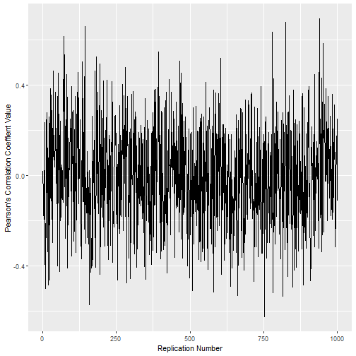

Not the pretties, but you get the idea. Correlation values are all over the place. How many times does the correlation value exceed the absolute value of .6?

testtot[[1]]

## [1] 5

Yep, 5 times. That’s fairly impressive. We were able to generate two random distributions, and depending on the sample, got correlation values that exceeded .6.

If you want to understand why a correlation coefficient doesn’t necessarily describe a real world relationship, this is why!

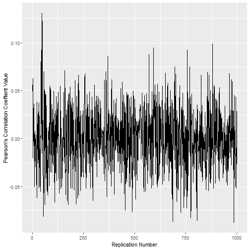
And if you want to play with some other numbers, say, with random distributions of size 1000 and do it a thousand times, we can.

test2 <- totfunc(1000, 1000, abs(.6))
 
test2[[1]]

## [1] 0

test2[[2]]