An Introduction to R: Data Cleaning, Wrangling, Visualizing, and Everything Else

# An Introduction to R: Data Cleaning, Wrangling, Visualizing, and Everything Else
## Part 3
### Daniel Katz

---

## Tidy data principles
#### The notion of tidy data comes from Hadley Wickham, the author of the tidyverse
+ The philosophy of tidy data shapes the tidyverse

1. Each variable has its own column
2. Each observation has its own row
3. Each value has its own cell
--

Because...
1. Uniformity makes everything easier and you know how your data is stored
1. It makes vectorization easier

However, sometimes we need both tidy forms, and non-tidyforms of data

---
Tidy (long data):
<table>
 <thead>
  <tr>
   <th style="text-align:left;"> country </th>
   <th style="text-align:right;"> year </th>
   <th style="text-align:right;"> cases </th>
   <th style="text-align:right;"> population </th>
  </tr>
 </thead>
<tbody>
  <tr>
   <td style="text-align:left;"> Afghanistan </td>
   <td style="text-align:right;"> 1999 </td>
   <td style="text-align:right;"> 745 </td>
   <td style="text-align:right;"> 19987071 </td>
  </tr>
  <tr>
   <td style="text-align:left;"> Afghanistan </td>
   <td style="text-align:right;"> 2000 </td>
   <td style="text-align:right;"> 2666 </td>
   <td style="text-align:right;"> 20595360 </td>
  </tr>
  <tr>
   <td style="text-align:left;"> Brazil </td>
   <td style="text-align:right;"> 1999 </td>
   <td style="text-align:right;"> 37737 </td>
   <td style="text-align:right;"> 172006362 </td>
  </tr>
  <tr>
   <td style="text-align:left;"> Brazil </td>
   <td style="text-align:right;"> 2000 </td>
   <td style="text-align:right;"> 80488 </td>
   <td style="text-align:right;"> 174504898 </td>
  </tr>
  <tr>
   <td style="text-align:left;"> China </td>
   <td style="text-align:right;"> 1999 </td>
   <td style="text-align:right;"> 212258 </td>
   <td style="text-align:right;"> 1272915272 </td>
  </tr>
  <tr>
   <td style="text-align:left;"> China </td>
   <td style="text-align:right;"> 2000 </td>
   <td style="text-align:right;"> 213766 </td>
   <td style="text-align:right;"> 1280428583 </td>
  </tr>
</tbody>
</table>

Not tidy (wide data):
<table>
 <thead>
  <tr>
   <th style="text-align:left;"> country </th>
   <th style="text-align:right;"> 1999 </th>
   <th style="text-align:right;"> 2000 </th>
  </tr>
 </thead>
<tbody>
  <tr>
   <td style="text-align:left;"> Afghanistan </td>
   <td style="text-align:right;"> 745 </td>
   <td style="text-align:right;"> 2666 </td>
  </tr>
  <tr>
   <td style="text-align:left;"> Brazil </td>
   <td style="text-align:right;"> 37737 </td>
   <td style="text-align:right;"> 80488 </td>
  </tr>
  <tr>
   <td style="text-align:left;"> China </td>
   <td style="text-align:right;"> 212258 </td>
   <td style="text-align:right;"> 213766 </td>
  </tr>
</tbody>
</table>
Years, here, are actually a value in their own right, thus values in a variable. Read more on the spread and gather functions, [here](https://r4ds.had.co.nz/tidy-data.html#spreading-and-gathering)

---
## Next functions go together, they're `group_by()` and `summarize()`

+ They do exactly what you think, but it's one of the more powerful tools in dplyr.

+ Let's use our `co16_rem` data.frame again

```r
names(co16_rem)
```

```
##  [1] "CDS"                        "Name"                      
##  [3] "AggLevel"                   "DFC"                       
##  [5] "Subgroup"                   "Subgrouptype"              
##  [7] "NumCohort"                  "NumGraduates"              
##  [9] "Cohort Graduation Rate"     "NumDropouts"               
## [11] "Cohort Dropout Rate"        "NumSpecialEducation"       
## [13] "Special Ed Completers Rate" "NumStillEnrolled"          
## [15] "Still Enrolled Rate"        "NumGED"                    
## [17] "GED Rate"                   "Year"
```
---
## The details
+ `group_by()` groups data together by some factor (such as class participation)

+ `summarize()` performs some operation on the grouped data, using summary statistics.

+ This is often useful for carrying out summary statistics-type analysis

---
## Let's get the average cohort size for males and females in a district

```r
mvf <- co16_rem %>% 
  select(CDS, DFC, AggLevel, Subgroup, Subgrouptype,
         NumCohort) %>% 
  filter(AggLevel=="D", 
         DFC=="N",
         Subgroup=="FEM"| Subgroup=="MAL",  
         Subgrouptype=="All")

## Sorry, this gets a little long.
## Can create as many vars as you want in summarize()
*mvf <-mvf %>% group_by(Subgroup) %>%
*     summarize(mean_co = mean(NumCohort, na.rm = T),
*           se = sd(NumCohort, na.rm = T))
```
<table>
 <thead>
  <tr>
   <th style="text-align:left;"> Subgroup </th>
   <th style="text-align:right;"> mean_co </th>
   <th style="text-align:right;"> se </th>
  </tr>
 </thead>
<tbody>
  <tr>
   <td style="text-align:left;"> FEM </td>
   <td style="text-align:right;"> 471.3473 </td>
   <td style="text-align:right;"> 961.308 </td>
  </tr>
  <tr>
   <td style="text-align:left;"> MAL </td>
   <td style="text-align:right;"> 491.6615 </td>
   <td style="text-align:right;"> 1007.660 </td>
  </tr>
</tbody>
</table>

---

## Challenge, `group_by()` and `summarize()`

1. Edit the code above so you're grouping by `Subgroup` AND `Subgrouptype` (feel free to use help).

2. However, with Subgroup, filter it first to include Male, Female, and "All".

3. Something the state of CA always looks at: Group by Subgrouptype such that we keep only those classified by CA as  
  + "Hispanic or Latinx" (5) 
  + "African American" (6)
  + "White, not Hispanic (7), and "All".

3. With as an outcome, instead of NumCohort, use NumGraduates

---
class: middle

# Solution

```r
mvf <- co16_rem %>% 
  select(CDS, DFC, AggLevel, Subgroup, Subgrouptype,
         NumGraduates) %>% 
  filter(AggLevel=="D", 
         DFC=="N",
         Subgroup=="MAL"| 
           Subgroup=="FEM"|
           Subgroup=="All"|
         Subgrouptype==5|
           Subgrouptype==6|
           Subgrouptype==7) %>% 
* group_by(Subgroup, Subgrouptype) %>%
  summarize(mean_grad = mean(NumGraduates, na.rm = T), 
            se = sd(NumGraduates, na.rm = T))
```
---
<table>
 <thead>
  <tr>
   <th style="text-align:left;"> Subgroup </th>
   <th style="text-align:left;"> Subgrouptype </th>
   <th style="text-align:right;"> mean_grad </th>
   <th style="text-align:right;"> se </th>
  </tr>
 </thead>
<tbody>
  <tr>
   <td style="text-align:left;"> All </td>
   <td style="text-align:left;"> 0 </td>
   <td style="text-align:right;"> 27.60000 </td>
   <td style="text-align:right;"> 23.69690 </td>
  </tr>
  <tr>
   <td style="text-align:left;"> All </td>
   <td style="text-align:left;"> 1 </td>
   <td style="text-align:right;"> 21.67797 </td>
   <td style="text-align:right;"> 21.83357 </td>
  </tr>
  <tr>
   <td style="text-align:left;"> All </td>
   <td style="text-align:left;"> 2 </td>
   <td style="text-align:right;"> 177.19718 </td>
   <td style="text-align:right;"> 281.27695 </td>
  </tr>
  <tr>
   <td style="text-align:left;"> All </td>
   <td style="text-align:left;"> 3 </td>
   <td style="text-align:right;"> 25.22807 </td>
   <td style="text-align:right;"> 21.12042 </td>
  </tr>
  <tr>
   <td style="text-align:left;"> All </td>
   <td style="text-align:left;"> 4 </td>
   <td style="text-align:right;"> 75.90964 </td>
   <td style="text-align:right;"> 111.06224 </td>
  </tr>
  <tr>
   <td style="text-align:left;"> All </td>
   <td style="text-align:left;"> 5 </td>
   <td style="text-align:right;"> 451.90408 </td>
   <td style="text-align:right;"> 1139.34147 </td>
  </tr>
</tbody>
</table>
---

```r
widemvf <- mvf %>% 
  gather(unit, numgrad, mean_grad:se) %>% 
  unite(temp1, Subgrouptype, unit, sep = ".") %>% 
  spread(temp1, numgrad)

head(widemvf) %>% 
  knitr::kable(format = "html")
```

<table>
 <thead>
  <tr>
   <th style="text-align:left;"> Subgroup </th>
   <th style="text-align:right;"> 0.mean_grad </th>
   <th style="text-align:right;"> 0.se </th>
   <th style="text-align:right;"> 1.mean_grad </th>
   <th style="text-align:right;"> 1.se </th>
   <th style="text-align:right;"> 2.mean_grad </th>
   <th style="text-align:right;"> 2.se </th>
   <th style="text-align:right;"> 3.mean_grad </th>
   <th style="text-align:right;"> 3.se </th>
   <th style="text-align:right;"> 4.mean_grad </th>
   <th style="text-align:right;"> 4.se </th>
   <th style="text-align:right;"> 5.mean_grad </th>
   <th style="text-align:right;"> 5.se </th>
   <th style="text-align:right;"> 6.mean_grad </th>
   <th style="text-align:right;"> 6.se </th>
   <th style="text-align:right;"> 7.mean_grad </th>
   <th style="text-align:right;"> 7.se </th>
   <th style="text-align:right;"> 9.mean_grad </th>
   <th style="text-align:right;"> 9.se </th>
   <th style="text-align:right;"> All.mean_grad </th>
   <th style="text-align:right;"> All.se </th>
  </tr>
 </thead>
<tbody>
  <tr>
   <td style="text-align:left;"> All </td>
   <td style="text-align:right;"> 27.60000 </td>
   <td style="text-align:right;"> 23.69690 </td>
   <td style="text-align:right;"> 21.67797 </td>
   <td style="text-align:right;"> 21.83357 </td>
   <td style="text-align:right;"> 177.1972 </td>
   <td style="text-align:right;"> 281.2770 </td>
   <td style="text-align:right;"> 25.22807 </td>
   <td style="text-align:right;"> 21.12042 </td>
   <td style="text-align:right;"> 75.90964 </td>
   <td style="text-align:right;"> 111.06224 </td>
   <td style="text-align:right;"> 451.9041 </td>
   <td style="text-align:right;"> 1139.3415 </td>
   <td style="text-align:right;"> 102.60396 </td>
   <td style="text-align:right;"> 196.9835 </td>
   <td style="text-align:right;"> 255.0025 </td>
   <td style="text-align:right;"> 354.4858 </td>
   <td style="text-align:right;"> 50.22034 </td>
   <td style="text-align:right;"> 51.38305 </td>
   <td style="text-align:right;"> 824.8698 </td>
   <td style="text-align:right;"> 1595.6264 </td>
  </tr>
  <tr>
   <td style="text-align:left;"> FEM </td>
   <td style="text-align:right;"> 25.80000 </td>
   <td style="text-align:right;"> 12.71613 </td>
   <td style="text-align:right;"> 23.13333 </td>
   <td style="text-align:right;"> 17.06654 </td>
   <td style="text-align:right;"> 101.8659 </td>
   <td style="text-align:right;"> 147.7555 </td>
   <td style="text-align:right;"> 21.26087 </td>
   <td style="text-align:right;"> 13.06006 </td>
   <td style="text-align:right;"> 46.50394 </td>
   <td style="text-align:right;"> 58.72560 </td>
   <td style="text-align:right;"> 257.5931 </td>
   <td style="text-align:right;"> 622.8693 </td>
   <td style="text-align:right;"> 67.14286 </td>
   <td style="text-align:right;"> 115.2403 </td>
   <td style="text-align:right;"> 145.5836 </td>
   <td style="text-align:right;"> 184.6204 </td>
   <td style="text-align:right;"> 34.07317 </td>
   <td style="text-align:right;"> 28.39567 </td>
   <td style="text-align:right;"> 443.6152 </td>
   <td style="text-align:right;"> 840.1522 </td>
  </tr>
  <tr>
   <td style="text-align:left;"> MAL </td>
   <td style="text-align:right;"> 23.42857 </td>
   <td style="text-align:right;"> 13.80649 </td>
   <td style="text-align:right;"> 22.25000 </td>
   <td style="text-align:right;"> 16.43776 </td>
   <td style="text-align:right;"> 104.0874 </td>
   <td style="text-align:right;"> 148.6343 </td>
   <td style="text-align:right;"> 22.04762 </td>
   <td style="text-align:right;"> 12.95946 </td>
   <td style="text-align:right;"> 48.98413 </td>
   <td style="text-align:right;"> 62.42858 </td>
   <td style="text-align:right;"> 236.5714 </td>
   <td style="text-align:right;"> 562.1065 </td>
   <td style="text-align:right;"> 61.48734 </td>
   <td style="text-align:right;"> 102.7873 </td>
   <td style="text-align:right;"> 143.9526 </td>
   <td style="text-align:right;"> 182.2362 </td>
   <td style="text-align:right;"> 33.30172 </td>
   <td style="text-align:right;"> 27.12522 </td>
   <td style="text-align:right;"> 423.9932 </td>
   <td style="text-align:right;"> 786.4833 </td>
  </tr>
</tbody>
</table>
---
# What if I want to know frequencies?
 + Can just do the same as above but use `n()`

```r
freqtab <- co16 %>%
  group_by(Subgroup, Subgrouptype) %>%
  summarise (n = n()) %>%
  mutate(freq = n / sum(n))
```

<table>
 <thead>
  <tr>
   <th style="text-align:left;"> Subgroup </th>
   <th style="text-align:left;"> Subgrouptype </th>
   <th style="text-align:right;"> n </th>
   <th style="text-align:right;"> freq </th>
  </tr>
 </thead>
<tbody>
  <tr>
   <td style="text-align:left;"> All </td>
   <td style="text-align:left;"> 0 </td>
   <td style="text-align:right;"> 740 </td>
   <td style="text-align:right;"> 0.0318705 </td>
  </tr>
  <tr>
   <td style="text-align:left;"> All </td>
   <td style="text-align:left;"> 1 </td>
   <td style="text-align:right;"> 1730 </td>
   <td style="text-align:right;"> 0.0745079 </td>
  </tr>
  <tr>
   <td style="text-align:left;"> All </td>
   <td style="text-align:left;"> 2 </td>
   <td style="text-align:right;"> 2249 </td>
   <td style="text-align:right;"> 0.0968603 </td>
  </tr>
  <tr>
   <td style="text-align:left;"> All </td>
   <td style="text-align:left;"> 3 </td>
   <td style="text-align:right;"> 1419 </td>
   <td style="text-align:right;"> 0.0611137 </td>
  </tr>
  <tr>
   <td style="text-align:left;"> All </td>
   <td style="text-align:left;"> 4 </td>
   <td style="text-align:right;"> 1830 </td>
   <td style="text-align:right;"> 0.0788148 </td>
  </tr>
  <tr>
   <td style="text-align:left;"> All </td>
   <td style="text-align:left;"> 5 </td>
   <td style="text-align:right;"> 3458 </td>
   <td style="text-align:right;"> 0.1489298 </td>
  </tr>
</tbody>
</table>
---

# Data VIZ with ggplot2

---
class: middle

## ggplot2

+ ggplot2 is a package built for visualizing all of our data.

+ I might say we've done things a little backwards

+ Start with data visualization

+ the general form of ggplot is:
`ggplot(data, aes(mapping)) + geom_function(aes(mappings))`
---

### Building a ggplot

1. Add an aesthetic internally or externally

1. Add a geome (what kind of plot will it be?)

1. Add other rules such as themes.

1. Get help via documentation or other resources as you need]

--
.pull-right[
1. `ggplot(data)`

1. `ggplot(data =df, aes(x=x_var, y=y_var))`

1. `ggplot(data=df, aes(x=x_var, y=y_var)) + geom_point(aes(color=grouo)) + geom_smooth(method=lm)`

1. `?ggplot2::geom_smooth`
]
---
class: middle, center

## Building a Plot

`ggplot(data=state16d, `
--
       `aes(x=droprate, y=GEDrate)) +`
--
         `geom_point()`

---
## Example

```r
ggplot(data=state16d, 
       aes(x=droprate, y=GEDrate)) + 
         geom_point(aes(color=Subgroup)) +
         geom_smooth(method = lm) 
```

---
## Logic of ggplot2
+ "An aesthetic is a visual property of the objects in your plot. Aesthetics include things like the size, the shape, or the color of your points."
  - Garrett Grolemund & Hadley Wickham in [R for Data Science](https://r4ds.had.co.nz/data-visualisation.html#aesthetic-mappings)

+ We have to make some decisions about how aesthetics should be mapped to your data.

+ What do we want our data to look like?

+ For instance, the x-axis aesthetic in the plot previously, was mapped to `Cohort Dropout Rate` and the color was mapped to `subgroup`

+ Other aesthetics include size and shape

+ It's important to know the `class` of your variables
---

# Another example
Just a histogram? (only one axis!)

```r
ggplot(data=state16d, 
       aes(x=NumCohort)) + 
  geom_histogram()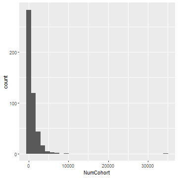
```

![](Intro_analysis_files/figure-html/unnamed-chunk-13-1.png)

---
## Warmup

```r
plot1 <- ggplot(data=state16d, 
                aes(x=droprate, y=GEDrate)) + 
         geom_point(aes(color=Subgroup))
```

1. What variables in state16d are categorical? Continuous? (hint, there's one command)

1. Using the code above, map a continuous variable to <mark>color</mark>, <mark>size</mark>, and <mark>shape</mark> (using geom_point). How do these aesthetics behave differently for categorical vs. continuous variables?

1. Use ?geom_point to find out what the `stroke` aesthetic does

1. instead of `color=Subgroup` above, use `color=GEDrate >.3`

1. What are three other `geom_functions`?

* These questions are modified versions of the ones found in _R for Data Science_
---

```r
plot1 <- ggplot(data=state16d, 
                aes(x=droprate, y=GEDrate)) + 
         geom_point(aes(color=GEDrate >.3))
```

---
# Challenge: Aesthetics
+ In California, Charter Schools are often continuation schools.

+ Much of the charter school debate doesn't really look at continuation schools, but they're not identified in our data

Using ggplot2, answer the questions:

+ Is there a relationship between the size of a school (NumCohort) and the grad rate (`Cohort Graduation Rate`)?

+ Does this relationship look different for charters and non-charter schools?

+ How might we visualize?

**Hint, The code for school level data for AggLevel = "S", Use subgroup and subgrouptype ="All", start with co16_rem and filter**

---

```r
# first, filter the data
graphdata2 <- state16 %>% 
  filter(AggLevel=="S", 
         Subgroup=="All", 
         Subgrouptype=="All")

# plot the data
plot2 <- ggplot(graphdata2, 
            aes(NumCohort, `Cohort Graduation Rate`))+
  geom_point(aes(color=DFC)) 
```

---
## We can also do this with pipes all the way through

```r
plot2 <- state16 %>% 
  filter(AggLevel=="S", 
         Subgroup=="All", 
         Subgrouptype=="All") %>%
  ggplot(aes(x=NumCohort, y=gradrate))+
  geom_point(aes(color=DFC))

plot2
```

---

## Using facets

+ Can we looked at the distributions of cohort sizes by non-charters and charters?

+ Can we answer the questions from the previous slides *within* charters and non-charters?

+ Absolutely, with facet_wrap

---

```r
plot3 <- ggplot(graphdata2, 
            aes(NumCohort))+
  geom_histogram() + facet_wrap(~DFC)

plot3
```

---
# Challenge: Facets
+ Facets use `~` which denotes a `formula.`

+ A formula is simply another data-structure in R. Don't worry about that, for now.

+ You can have two sides to the formula. To see this, run the code:

```r
graphdata3 <- state16 %>% 
  filter(AggLevel=="S", 
         Subgroup=="MAL"| Subgroup=="FEM", 
         Subgrouptype=="All")

plot4 <- ggplot(graphdata3, 
            aes(NumDropouts))+
  geom_histogram() + facet_wrap(~Subgroup, nrow=1)

#vs

plot5 <- ggplot(graphdata3, 
            aes(NumDropouts))+
  geom_histogram() + facet_wrap(DFC~Subgroup)
```
---
# Plot 4

```r
plot4
```

---
# Plot 5

```r
plot5
```

<img src="Intro_analysis_files/figure-html/unnamed-chunk-21-1.png" style="display: block; margin: auto;" />
---
class: middle
# What happens when you replace facet_wrap with facet_grid?

```r
plot6 <- ggplot(graphdata3, 
            aes(NumDropouts))+
  geom_histogram() + 
  facet_grid(DFC~Subgroup)
```
---

```r
plot6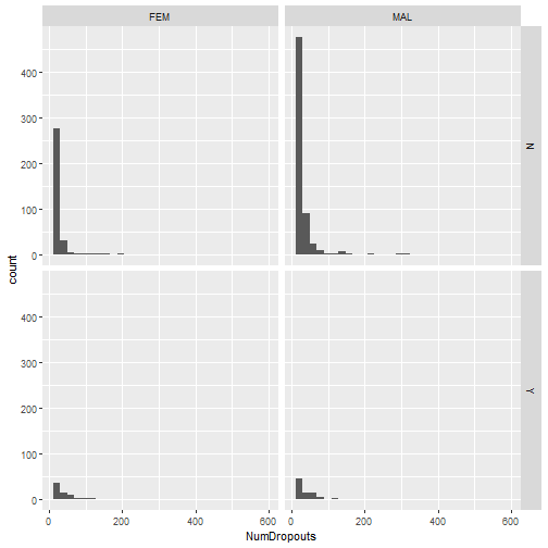
```

![](Intro_analysis_files/figure-html/unnamed-chunk-23-1.png)

---
class: middle

## More on `geom_`
+ According to Hadley Wickham, author of ggplot2, `geom_s` are so-called because they represent the geometric objects that we use to represent data

+ Boxplots use <mark>box geoms</mark>, line charts use <mark>line geoms</mark>, scatter plots use...

--
  + Point geoms
  
--
  
+ We can represent the same data in multiple ways using geoms_

+ we've already played with geoms above, to get a sense.

+ Because of code completion, with `geom_ ` in a function, we can see our options.
---

## Geoms continued

+ we can add aesthetics just to that `geom_function`

```r
plot7 <- ggplot(graphdata3, 
            aes(x=NumDropouts, y = gradrate))+
  geom_point(aes(color=Subgroup))

plot7
```

---

## Challenge (geoms)

1. Make a boxplot starting with `state16` data creating `graphdata4` by
  1.  filtering so `subgrouptype` = "All"
  1. `Subgroup` = "MAL", "FEM" and "All"
  1. looking at the difference between graduation rates (gradrates) for charters and non-charters, but just

2. Add a group to the boxplot such that you look at differences between charters and non-charters and the subgroups (using `Subgroup`) within each

--
1. Start with:

```r
graphdata4 <- state16 %>% 
  filter(Subgroup=="MAL"| Subgroup=="FEM"|Subgroup=="All", 
         Subgrouptype=="All")
```

---
## Solutions

```r
#bar chart
ggplot(graphdata4) + 
  geom_boxplot(aes(y = gradrate, x = DFC,
*                  fill="red"))
```

---

```r
#bar chart
ggplot(graphdata4, 
       aes(y = gradrate, x = DFC, fill = Subgroup)) +
*      geom_boxplot()
```

---

## All the geoms
There are a lot of geoms_

See the most popular geoms, [_**here**_](https://eric.netlify.com/2017/08/10/most-popular-ggplot2-geoms/)

---
## Starting to think about descriptives, putting it together

+ Faceting is super useful when you want to look at correlations by group. Go back to `graphdata4`

```r
plotcorr <- ggplot(graphdata4, 
            aes(x=droprate, y = gradrate))+
  geom_point(aes(color=Subgroup)) + 
  facet_grid(Subgroup~DFC) 
```
---

```r
plotcorr
```

---
## ggplot2 Labels

+ ggplot2 objects can be always added to with a `+`

+ What we'll add is `labs()`

```r
plotcorr <- plotcorr + 
* labs(y="Cohort Graduation Rate",
  x= "Cohort Dropout Rate", 
  title = "Relationship between hs grad rates and dropout rates")

plotcorr
```

<img src="Intro_analysis_files/figure-html/unnamed-chunk-30-1.png" style="display: block; margin: auto;" />
---

### Challenge: Using labs,

1. Add a subtitle to the plot 
1. Change the order of the facet/rearrange the facet using facet_grid(x~y)
---
#solution (labs)

```r
plotcorr <- ggplot(graphdata4, 
            aes(x=droprate, y = gradrate))+
  geom_point(aes(color=Subgroup)) + 
  facet_grid(DFC~Subgroup) +
* labs(y="Cohort Graduation Rate",
  x= "Cohort Dropout Rate", 
  title = "Relationship between hs grad rates and dropout rates",
  subtitle = "As faceted by CA subgroup and charter status")

plotcorr
```

<img src="Intro_analysis_files/figure-html/unnamed-chunk-31-1.png" style="display: block; margin: auto;" />
---
## What about changing the legened?
This is a good resource for more on [_**ggplot text**_](http://r-statistics.co/Complete-Ggplot2-Tutorial-Part2-Customizing-Theme-With-R-Code.html):

```r
plotcorr <- plotcorr +  
  scale_color_discrete(labels = c("All", "Female", "Male"))
plotcorr
```

---
## Labelling individual Cases (with GEDrates greater than 20%)
See package, [_**ggrepl**_](https://cran.r-project.org/web/packages/ggrepel/vignettes/ggrepel.html) to make this cleaner

```r
plotlab <- plot1 +  geom_text(data=subset(graphdata4, GEDrate >30), 
          aes(x=droprate, y = GEDrate, label=Name))
          
plotlab
```

<img src="Intro_analysis_files/figure-html/unnamed-chunk-33-1.png" style="display: block; margin: auto;" />
---
# There's much, much, much more:

+ Check out themes related to ggplot2

+ Check out how to make plots APA or the like, compliant here: [_**APA**_](https://ndphillips.github.io/IntroductionR_Course/assignments/wpa/wpa_5.html)

+ A good startin place, as usual, is the ggplot2 R studio [_**page**_](https://ggplot2.tidyverse.org/)

---
# Exporting data/saving data

+ To export data from R is quite simple, but remember our directories!

+ We want to put any data we've cleaned in a folder called something like, "cleaneddata" and give it a name so we know what's in there. 
---

+ Remember `state16d`?

+ We'll use the `write_csv()` function from the `readr` package.

+ general form (`write_csv(df, "folder/data.csv1"`) - extension can be anything related to `write_*` start typing `write_` to see what happens...

+ What you save it as (in quotes) doesn't have to be the same as what it's called in R.

```r
write_csv(state16d, "Cleandata/districtsub.csv")

# to write to SPSS
library(haven)
write_sav(state16d, "Cleandata/districtsub.sav")

# sav is an SPSS file extension
```
---

# Exporting ggplot2 object

```r
ggsave("plot1.pdf", plot1)

ggsave("plot1.png", plot1)

# make it a certain size
ggsave("plot1.png", width = 20, height = 20, units = "cm")
```
---

1. Export one dataframe you made, either in csv or SPSS file format to a "wrangledata" subdirectory in your working directory

1. Export one plot you made to a folder called `plots` in your working directory.

---

# Part 3.2: Descriptive statistics
+ One of the best asepcts of R is that there are a lot of ways to do the same thing.

--
+ This is also one of the worst aspects of R

+ We've already seen a few ways to get descriptive statistics just brute forcing it with dplyr.

---

#### Workflow: Explore, Visualize, Describe, Model

<img src="datasciexp.png" width="689" style="display: block; margin: auto;" />
---
## An easy way to get descriptives
+ Remember `summary()`

+ What happens when you run `summary()` on all of state16d?

+ What happens when you run `summary()` on just one column?

```r
summary(state16d)
```

```
##      CDS                Name             AggLevel             DFC           
##  Length:493         Length:493         Length:493         Length:493        
##  Class :character   Class :character   Class :character   Class :character  
##  Mode  :character   Mode  :character   Mode  :character   Mode  :character  
##                                                                             
##                                                                             
##                                                                             
##                                                                             
##    Subgroup         Subgrouptype         NumCohort        NumGraduates    
##  Length:493         Length:493         Min.   :   11.0   Min.   :   11.0  
##  Class :character   Class :character   1st Qu.:  134.0   1st Qu.:  119.0  
##  Mode  :character   Mode  :character   Median :  372.0   Median :  336.0  
##                                        Mean   :  922.1   Mean   :  824.9  
##                                        3rd Qu.: 1108.8   3rd Qu.: 1021.0  
##                                        Max.   :34472.0   Max.   :26654.0  
##                                        NA's   :19        NA's   :32       
##   NumDropouts        gradrate         droprate        GEDrate       
##  Min.   :  11.0   Min.   :  0.00   Min.   : 0.00   Min.   : 0.0000  
##  1st Qu.:  25.0   1st Qu.: 84.21   1st Qu.: 2.90   1st Qu.: 0.0000  
##  Median :  49.0   Median : 90.91   Median : 5.50   Median : 0.0000  
##  Mean   : 106.7   Mean   : 83.38   Mean   :10.21   Mean   : 0.2079  
##  3rd Qu.: 115.0   3rd Qu.: 94.81   3rd Qu.:10.00   3rd Qu.: 0.0000  
##  Max.   :4738.0   Max.   :100.00   Max.   :81.10   Max.   :15.7000  
##  NA's   :184
```

```r
summary(state16d$NumGraduates)
```

```
##    Min. 1st Qu.  Median    Mean 3rd Qu.    Max.    NA's 
##    11.0   119.0   336.0   824.9  1021.0 26654.0      32
```

+ Both give us NAs, which is convenient

+ Can also build from scratch using xtable

+ But hard to export (I still use these to get a quick understanding)
---

## I personally like the Startgazer package

+ `Stargazer` will give you descriptive statistics that are outputtable

+ `Stargazer` will output to various styles (problematically, no apa style option, though, but close enough)

+ `Stargazer` will format your regression output (as we'll see)

+ For writing in word
  + I recommend html output
  because you can open it with Excel and edit or open in webbrowser and copy-paste into spreadsheet
  + Can also output to Latex

+ Stargazer takes as argument the data (or the data subset), the way to output the data, and many others (see ?Stargazer)

+ The challenge with stargazer is that you need to make sure the dataframe is of class, data.frame (you have to coerce it, see below)

---
## Example

```r
library(stargazer)

# Need to select only numeric vars
numdist <- state16d %>% 
  select(NumCohort:GEDrate) %>% 
  as.data.frame(.)

stargazer(numdist, type="html", 
          out = "describe.html", 
          digits = 2)
```

```
## 
## <table style="text-align:center"><tr><td colspan="8" style="border-bottom: 1px solid black"></td></tr><tr><td style="text-align:left">Statistic</td><td>N</td><td>Mean</td><td>St. Dev.</td><td>Min</td><td>Pctl(25)</td><td>Pctl(75)</td><td>Max</td></tr>
## <tr><td colspan="8" style="border-bottom: 1px solid black"></td></tr><tr><td style="text-align:left">NumCohort</td><td>474</td><td>922.07</td><td>1,934.79</td><td>11.00</td><td>134.00</td><td>1,108.75</td><td>34,472.00</td></tr>
## <tr><td style="text-align:left">NumGraduates</td><td>461</td><td>824.87</td><td>1,595.63</td><td>11.00</td><td>119.00</td><td>1,021.00</td><td>26,654.00</td></tr>
## <tr><td style="text-align:left">NumDropouts</td><td>309</td><td>106.65</td><td>289.38</td><td>11.00</td><td>25.00</td><td>115.00</td><td>4,738.00</td></tr>
## <tr><td style="text-align:left">gradrate</td><td>493</td><td>83.38</td><td>21.52</td><td>0.00</td><td>84.21</td><td>94.81</td><td>100.00</td></tr>
## <tr><td style="text-align:left">droprate</td><td>493</td><td>10.21</td><td>14.06</td><td>0.00</td><td>2.90</td><td>10.00</td><td>81.10</td></tr>
## <tr><td style="text-align:left">GEDrate</td><td>493</td><td>0.21</td><td>1.19</td><td>0.00</td><td>0.00</td><td>0.00</td><td>15.70</td></tr>
## <tr><td colspan="8" style="border-bottom: 1px solid black"></td></tr></table>
```
---

## Challenge, descriptive statistics

1.  Using stargazer documentation, change the "type" argument so that it outputs in a way that you can understand the output either in the console or the viewer.

2. Using stargazer documentation, change the table "title."

3. How can you use the `flip` argument?

---
## Solutions

```r
stargazer(numdist, type="text", 
          digits = 2, 
          title = "Danny's Descriptive Statistics")
```

```
## 
## Danny's Descriptive Statistics
## ==================================================================
## Statistic     N   Mean  St. Dev.  Min  Pctl(25) Pctl(75)    Max   
## ------------------------------------------------------------------
## NumCohort    474 922.07 1,934.79 11.00  134.00  1,108.75 34,472.00
## NumGraduates 461 824.87 1,595.63 11.00  119.00  1,021.00 26,654.00
## NumDropouts  309 106.65  289.38  11.00  25.00    115.00  4,738.00 
## gradrate     493 83.38   21.52   0.00   84.21    94.81    100.00  
## droprate     493 10.21   14.06   0.00    2.90    10.00     81.10  
## GEDrate      493  0.21    1.19   0.00    0.00     0.00     15.70  
## ------------------------------------------------------------------
```

```r
stargazer(numdist, type="text", 
          digits = 2, 
          title = "Danny's Descriptive Statistics",
          flip = T)
```

---

#Describeby, with `psych`

+ Another useful descriptive statistics package is `psych` which also has a lot of other useful tools including, various psychometric-type analysis functions

+ It provides descriptive statistics by a certain grouping variable\

+ Run the code below and also replace `mat=T` with `mat=F`

+ What happens?

---

```r
library(psych)

numdist2 <- state16 %>%
  select(DFC, 
         Subgroup, 
         Subgrouptype, 
         NumCohort:GEDrate) 
    
numdist2 <- numdist2 %>% 
  filter(Subgroup=="All"|Subgrouptype=="All")%>%
  as.data.frame(.) %>% 
  select(-Subgroup, -Subgrouptype)

# This is the actual psych package code
descriptab <- describeBy(numdist2, 
                          group = numdist2$DFC, 
                          na.rm=T, 
                         digits = 2)
```

---

Class: middle

## Aside, lists...

+ We haven't touched lists, but many packages will output in list form

+ That is, it'll give you a `list` of output.

+ In the `Global Environment`, if you click on the blue arrow next to a list, it'll show you the list elements.

+ You can also use `str(list_name)`

---

Class: middle

# Examples

+ A list can contain other data structures.

+ What does `descriptab$Y` do? What about `descrptab[[1]]`?
--

```r
str(descriptab)
descriptab$Y
descriptab[[1]]
```

+ You can view package output by viewing the documentation (output is described in `Values` section of documentation)

+ You can access package output by using
  + `object$name` like above, 
  + or `object[[1]]` where the 1 is replaced with the desired position and double brackets represents position in the list.

+ No shortcut, here, just have to read the documentation

---

Class: middle

# Wrapping up descriptives

+ For nice correlation output, please check out the `apaTables` package

+ For quick output, check Hmisc

+ Don't forget the tidyverse!

+ An overview of the descriptive statistics methods [_**here**_](https://dabblingwithdata.wordpress.com/2018/01/02/my-favourite-r-package-for-summarising-data/)

---
class: middle

## Some basic linear models

+ The basic linear models from R, require no external packages.

+ R was built for statistics!

We'll look at two main statistical tools, today...

+ `t.test` and `lm()` (anything else you all want to see?)

+ Other options include paired sample t.test, different alternative hypotheses

---
Class: middle

## `t tests`
+ t-tests in R are run simply by using `t.test()`

+ `?t.test`, you'll want "stats::t.test"

+ R assumes, unequal variances of the two groups, thus uses Welch's test

+ However, this is just a little more stringent. To override, use, `var.equal=T`

+ If your two factors are in two different columns, you might need to name them (remember tidydata is easier)
---
# Example run code, below:

```r
# this creates fictional data
NYCtestscore <- rnorm(1000, mean = 2, sd=1)
LAtestscore <- rnorm(1000, mean = 3, sd=1)
testscores <- cbind(NYCtestscore, LAtestscore)
head(testscores)
```

```
##      NYCtestscore LAtestscore
## [1,]    2.7349779    4.165935
## [2,]    2.6011543    4.565074
## [3,]    0.4261416    2.630528
## [4,]    1.8561137    2.691927
## [5,]    1.1962862    2.759620
## [6,]    2.3860276    4.826200
```

```r
# two group
mod1 <- t.test(NYCtestscore, LAtestscore)
```

---
class: middle

```r
mod1
```

```
## 
## 	Welch Two Sample t-test
## 
## data:  NYCtestscore and LAtestscore
## t = -22.825, df = 1992.8, p-value < 2.2e-16
## alternative hypothesis: true difference in means is not equal to 0
## 95 percent confidence interval:
##  -1.136012 -0.956246
## sample estimates:
## mean of x mean of y 
##  1.989207  3.035336
```
---

## Easier, using a formula,, but only applicable using two-sample test
+ If your factor is in one column (such as charter/not charter in DFC)

+ Takes the form `t.test(state16, Outcome~Factor)`

+ Try doing this with `state16`, using gradrate and DFC

+ You can access different parts of the t.test if you use `mod2$*`
---
## The Broom Package
+ Also, check out the `broom` package and the function `tidy`

```r
library(broom)
mod2 <- t.test(data=state16, gradrate~DFC)

tidy(mod2)
```

```
## # A tibble: 1 x 10
##   estimate estimate1 estimate2 statistic   p.value parameter conf.low conf.high
##      <dbl>     <dbl>     <dbl>     <dbl>     <dbl>     <dbl>    <dbl>     <dbl>
## 1     10.2      75.7      65.5      30.1 6.66e-195    19784.     9.56      10.9
## # ... with 2 more variables: method <chr>, alternative <chr>
```

---

class: middle 
## Linear regression
+ The form is `lm(outcome ~ covariate1 + covariat2...)`
  + Where lm() is the regression function

+ You can use stargazer to output nice tables

+ You can easily check assumptions, visually

+ You don't need to dummy out categorical variables as long as they're factors (or, at least, character)

+ You can interact variables within the equation with `*`,

`lm(outcome ~ covariate1 + covariate2 + covariate1* covariat2)`

or `:`

`lm(outcome ~ covariate1 + covariate2 + covariate1: covariat2)`
---
# Linear Regression
`$\widehat{gradraterate} = \alpha + \beta_1DFC$`

```r
# Example usage
modlm1 <- lm(data = state16, gradrate~DFC)
summary(modlm1)
```

```
## 
## Call:
## lm(formula = gradrate ~ DFC, data = state16)
## 
## Residuals:
##    Min     1Q Median     3Q    Max 
## -75.70 -15.70  16.30  24.30  34.53 
## 
## Coefficients:
##             Estimate Std. Error t value Pr(>|t|)    
## (Intercept)  75.7028     0.1371  552.17   <2e-16 ***
## DFCY        -10.2287     0.3152  -32.45   <2e-16 ***
## ---
## Signif. codes:  0 '***' 0.001 '**' 0.01 '*' 0.05 '.' 0.1 ' ' 1
## 
## Residual standard error: 33.87 on 75260 degrees of freedom
## Multiple R-squared:  0.0138,	Adjusted R-squared:  0.01379 
## F-statistic:  1053 on 1 and 75260 DF,  p-value: < 2.2e-16
```
---
# It's easy to check assumptions

```r
# to check assumptions
plot(modlm1)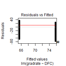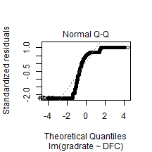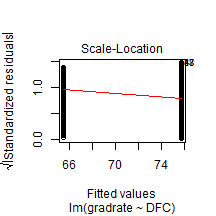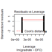
```

![](Intro_analysis_files/figure-html/unnamed-chunk-49-1.png)![](Intro_analysis_files/figure-html/unnamed-chunk-49-2.png)![](Intro_analysis_files/figure-html/unnamed-chunk-49-3.png)![](Intro_analysis_files/figure-html/unnamed-chunk-49-4.png)

---
class: middle

# Challenge

1.  Run a regression in which you regress GEDrate on droprate and DFC using state16 data:

+ filter subgrouptype="All"
  + filter AggLevel!="T"
  
.center[$\widehat{GEDrate} = \alpha +\beta_1droprate + \beta_2DFC$]

1. Regress GEDrate on droprate as well as the interaction term between DFC and Subgroup 
`$\widehat{GEDrate} = \alpha + \beta_1droprate + \beta_2DFC + \beta_3DFC*Subgroup$`

1. Interpret results (roughly)
---

```r
state16_2 <- state16 %>%
  filter(Subgrouptype=="All",
         AggLevel!="T")

mod3 <- lm(data=state16_2, GEDrate~droprate + DFC)
mod4 <- lm(data=state16_2, GEDrate~droprate + DFC*Subgroup)
```

---
# Ugly...

```r
summary(mod3)
```

```
## 
## Call:
## lm(formula = GEDrate ~ droprate + DFC, data = state16_2)
## 
## Residuals:
##    Min     1Q Median     3Q    Max 
## -0.416 -0.195 -0.159 -0.146 99.854 
## 
## Coefficients:
##               Estimate Std. Error t value Pr(>|t|)    
## (Intercept)  0.1460687  0.0166196   8.789  < 2e-16 ***
## droprate     0.0027041  0.0005437   4.974 6.61e-07 ***
## DFCY        -0.0458140  0.0313436  -1.462    0.144    
## ---
## Signif. codes:  0 '***' 0.001 '**' 0.01 '*' 0.05 '.' 0.1 ' ' 1
## 
## Residual standard error: 1.866 on 22236 degrees of freedom
## Multiple R-squared:  0.001184,	Adjusted R-squared:  0.001094 
## F-statistic: 13.18 on 2 and 22236 DF,  p-value: 1.901e-06
```

```r
summary(mod4)
```

```
## 
## Call:
## lm(formula = GEDrate ~ droprate + DFC * Subgroup, data = state16_2)
## 
## Residuals:
##    Min     1Q Median     3Q    Max 
## -0.500 -0.231 -0.179 -0.103 99.846 
## 
## Coefficients:
##                    Estimate Std. Error t value Pr(>|t|)    
## (Intercept)       0.1793643  0.0357456   5.018 5.27e-07 ***
## droprate          0.0026937  0.0005447   4.945 7.66e-07 ***
## DFCY             -0.0587284  0.0771780  -0.761  0.44670    
## SubgroupEL       -0.0257836  0.0507687  -0.508  0.61155    
## SubgroupFEM      -0.0857560  0.0496538  -1.727  0.08417 .  
## SubgroupMAL       0.0515013  0.0492089   1.047  0.29530    
## SubgroupMIG      -0.1834390  0.0645977  -2.840  0.00452 ** 
## SubgroupSD        0.0114432  0.0492309   0.232  0.81620    
## SubgroupSE       -0.0918579  0.0496466  -1.850  0.06429 .  
## DFCY:SubgroupEL  -0.0750446  0.1128792  -0.665  0.50617    
## DFCY:SubgroupFEM  0.0408527  0.1096171   0.373  0.70939    
## DFCY:SubgroupMAL  0.0005511  0.1094213   0.005  0.99598    
## DFCY:SubgroupMIG -0.0084742  0.1623642  -0.052  0.95838    
## DFCY:SubgroupSD  -0.0350583  0.1092513  -0.321  0.74829    
## DFCY:SubgroupSE   0.1301154  0.1112262   1.170  0.24208    
## ---
## Signif. codes:  0 '***' 0.001 '**' 0.01 '*' 0.05 '.' 0.1 ' ' 1
## 
## Residual standard error: 1.866 on 22224 degrees of freedom
## Multiple R-squared:  0.002343,	Adjusted R-squared:  0.001715 
## F-statistic: 3.729 on 14 and 22224 DF,  p-value: 2.65e-06
```
---
# Better!

```r
stargazer(mod3, mod4, type = "text", out = "modcompare.html")
```

```
## 
## =======================================================================
##                                     Dependent variable:                
##                     ---------------------------------------------------
##                                           GEDrate                      
##                                (1)                       (2)           
## -----------------------------------------------------------------------
## droprate                    0.003***                  0.003***         
##                              (0.001)                   (0.001)         
##                                                                        
## DFCY                         -0.046                    -0.059          
##                              (0.031)                   (0.077)         
##                                                                        
## SubgroupEL                                             -0.026          
##                                                        (0.051)         
##                                                                        
## SubgroupFEM                                            -0.086*         
##                                                        (0.050)         
##                                                                        
## SubgroupMAL                                             0.052          
##                                                        (0.049)         
##                                                                        
## SubgroupMIG                                           -0.183***        
##                                                        (0.065)         
##                                                                        
## SubgroupSD                                              0.011          
##                                                        (0.049)         
##                                                                        
## SubgroupSE                                             -0.092*         
##                                                        (0.050)         
##                                                                        
## DFCY:SubgroupEL                                        -0.075          
##                                                        (0.113)         
##                                                                        
## DFCY:SubgroupFEM                                        0.041          
##                                                        (0.110)         
##                                                                        
## DFCY:SubgroupMAL                                        0.001          
##                                                        (0.109)         
##                                                                        
## DFCY:SubgroupMIG                                       -0.008          
##                                                        (0.162)         
##                                                                        
## DFCY:SubgroupSD                                        -0.035          
##                                                        (0.109)         
##                                                                        
## DFCY:SubgroupSE                                         0.130          
##                                                        (0.111)         
##                                                                        
## Constant                    0.146***                  0.179***         
##                              (0.017)                   (0.036)         
##                                                                        
## -----------------------------------------------------------------------
## Observations                 22,239                    22,239          
## R2                            0.001                     0.002          
## Adjusted R2                   0.001                     0.002          
## Residual Std. Error    1.866 (df = 22236)        1.866 (df = 22224)    
## F Statistic         13.181*** (df = 2; 22236) 3.729*** (df = 14; 22224)
## =======================================================================
## Note:                                       *p<0.1; **p<0.05; ***p<0.01
```

---
# Challenge:
**Try to plot mod3 in ggplot2**
--
Careful in interpretation (make a scatter plot or add points if you'd like)

```r
ggplot(data=state16_2, 
        aes(x=droprate, y=GEDrate, color=DFC)) +
  geom_smooth(method = lm) +
  labs(x="Dropout Rate (%)",
       y = "GED Rate (%)")
```

<img src="Intro_analysis_files/figure-html/unnamed-chunk-53-1.png" style="display: block; margin: auto;" />
---

## Data Cleaning and Modelling Tips

1. Always get a sense of your data first. 
  + Dipstick: Take a sample of a few cases, how do they look? As you'd expect?
  + Visualize and describe
  
1. After any transformation, make sure to compare a few cases in the raw data and the new data. 
  + use visualization to compare raw data and cleaned data.
  + Do they look right?
  
1. Careful, make sure your factors and or factors

1. Do your model results strain credulity? Too good to be true?
  + Use visualization to make sure there aren't weird cases
  + use descriptives

1. If you do any merging, take the "Dipstick" approach. 
  
1. If there's somebody you can work with, have them look at your code!

---
# Getting help in R

+ First, I hope this has been helpful.

+ I've posted a list of resources here: [**_Helplist_**](/help/helplist.html)

+ Next, please continue working at it. Today was probably really overwhelming.

+ There are a lot of R resources out there!
---
## What should I continue to learn?

+ Overall, data management and cleaning (remember, tidy!)

+ Spreading and gathering from tidyr (soon to be [pivot_longer and pivot_wider](https://tidyr.tidyverse.org/dev/articles/pivot.html)

+ merging data with the [join functions from dply](https://dplyr.tidyverse.org/reference/join.html) and merging data by row (for example, long data) with [bind_rows](https://dplyr.tidyverse.org/reference/bind.html)

+ Check out how matrices work

+ Find something you need to do - do it

+ The joy of R is in writing functions and iteration.
---
## Finding help with Google

+ You'll often find "vignettes" - these are documents that people, often package authors, have created to give some in-depth examples.

+ You'll find the package documentation

+ You'll find other examples from classes, blogs, etc.

+ You'll find...Stack Exchange/Stack Overflow, and you will use it!

---

## How to use Stack Overflow/Stack Exchange

+ Usual Scenario: Trying to do something, can't figure it out.

+ You Google it and find a number of posts about your topic. You settle on one and there are a bunch of answers.

+ Which one is right? Which one is best?

+ Usually, there are a few routes to your solution
---

## Posts (try to find the most recent)

---

## Upvotes (Good Question)

---
class: middle

***Answers (which one has the most upvotes? Which one matches)***

---
class: middle

***People liked the answer from the previous slide but it's old, might be a solution: Scroll through non-featured***
<img src="scroll.jpg" width="1647" style="display: block; margin: auto;" />
---

***A featured new answer, but not as many upvotes! A solution and link!***
<img src="newgood.jpg" width="1792" style="display: block; margin: auto;" />
---

## Github

+ All R packages that are on `CRAN` have to be posted on Github

+ If you Google a package name, it's Github page comes up

+ Github is a project tracking/version control page where people can track and share projects.

+ The R code here is usually the source code that makes a package work.
--
+ You rarely want this unless you want to know why you're getting some error and are maybe ready to scroll [*through lots and lots of code...*](https://github.com/philchalmers/mirt/blob/master/R/EMstep.utils.R)

+ But it **can** be [_**useful at times!**_](https://github.com/philchalmers/mirt/wiki)
---

## Any other questions? Concerns?